Hash Join
Overview
Basic idea:
- Use hashing to partition relations.
- To avoid having to consider all pairs of tuples.
Requires sufficient memory buffers:
- To hold substantial portions of partitions.
- (Preferably) to hold largest partition of outer relation.
Other issues:
- Works only for equijoin.
- Susceptible to data skew (or poor hash function).
Variations: simple, grace, hybrid.
Simple Hash Join
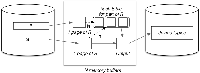
Basic approach:
- Hash part of outer relation
Rinto memory buffers (build). - Scan inner relation
S, using hash to search (probe).- If
R.i = S.j, thenh(R.i) = h(S.h)(hash to same buffer). - Only need to check one memory buffer for each
Stuple.
- If
- Repeat until whole of
Rhas been processed.
No overflows allowed in in-memory hash table:
- Works best with uniform hash function.
- Can be adversely affected by data/hash skew.
Algorithm Implementation
For Join[R.i=S.j](R, S):
for r in R:
    # don't allow overflows.
    # flush once buffers are full.
    if buffer[h(r.i)].isFull():
        for s in S:
            for rr in buffer[h(s.j)]:
                if satisfiesJoin(rr, s):
                    # add (Rr, s) to result
        # clear all hash table buffers

    buffer[h(R.i)].insert(r)
Cost
Best case: all tuples of R fit in the hash table:
- Cost =
b_R + b_S. - Same page reads as block nested loop, but less join tests.
Good case: refill hash table m times (where m >= ceil(b_R / (N - 3))):
- Cost =
b_R + m * b_S. - More page reads than block nested loop, but less join tests.
Worst case: everything hases to same page:
- Cost =
b_R + b_R * b_S.
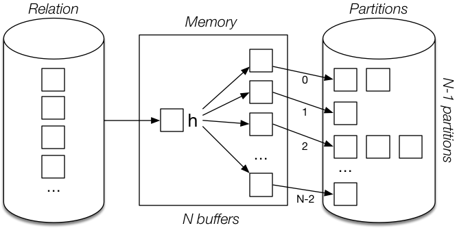
Grace Hash Join
Basic approach:
- Partition both relations on join attribute using hashing (
h1). - Load each partition of
Rinto(N - 3)buffers hash table(h2). - Scan through corresponding partition of
Sto form results. - Repeat until all partitions exhausted.
Partition phase (applied to both R and S):
Probe/join phase:

The second hash function (h2) speeds up matching process. Without it, would need to scan entire R partition for each record in S partition.
Cost of Grace Hash Join
- Number of pages in all partition files of Rel ~=
b_Rel(maybe slightly more). - Partition relations:
- Cost =
read(b_R) + write(~=b_R) = 2b_R. - Similarly for
S.
- Cost =
- Probe/join requires one scan of each partitioned relation:
- All hashing and comparison occurs in memory ==> tiny cost.
Total cost = 2b_R + 2b_S + b_R + b_S = 3(b_R + b_S).
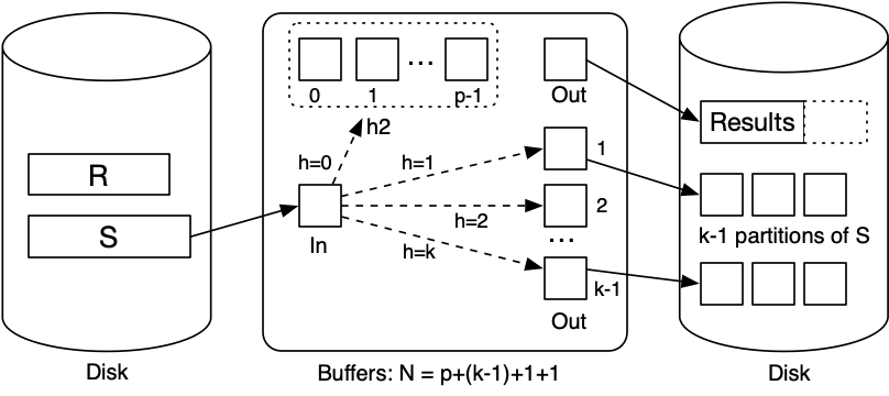
Hybrid Hash Join
Variant of grace hash join if we have sqrt(b_R) < N < b_r + 2 buffers.
- Create
k << Npartitions, 1 in memory,k - 1on disk. - Buffers: 1 input,
k - 1output,p = N - k - 2for in-memory partition.
When we come to scan and partition S relation:
- Any tuple with hash 0 can be resolved using in-memory partition.
- Other tuples are written to one of
k - 1partition files forS.
Final phase is same as grace join, but with only k - 1 partitions.
Comparison:
- Grace hash join creates
N - 1partitions on disk. - Hybrid hash join creates
1(memory) +k - 1(disk) partitions.
Phase 1: partition R:

Phase 2: partition S:
Phase 3: finishing join (same as grace join):
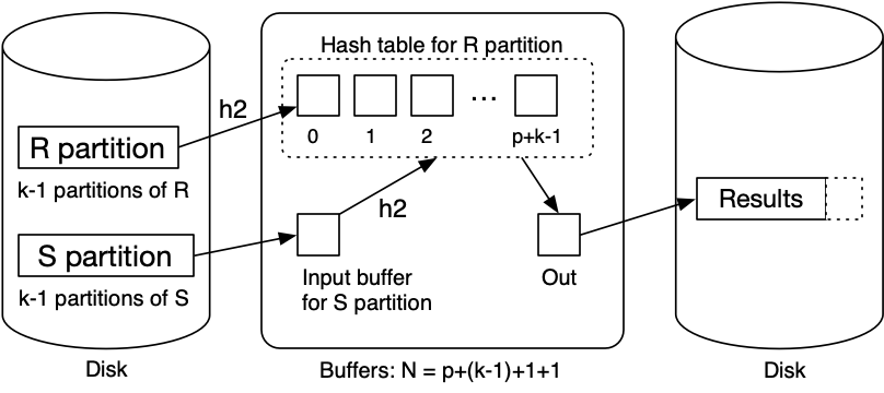
Observations:
- With
kpartitions, each partition has expected sizeceil(b_R / k). - Holding 1 partition in memory needs
ceil(b_R / k)buffers. - Trade-off between in-memory partition space and number of partitions.
Other notes:
- If
N = b_R + 2, using block nested loop join is simpler. - Cost depends on
N(but less than grace hash join).
For k partitions, Cost = (3 - 2 / k) * (b_R + b_S).