Query Optimisation

Overview

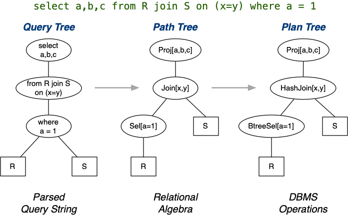
The query optimiser:

Takes RA expression from SQL compiler.
Produces sequence of RelOps to evaluate the expression.

Optimisers aim to find a good plan, but maybe not optimal.

Observed query time = planning time + evaluation time.
- Limited planning time means we can’t always find optimal plan.
  - Would require exhaustive search of very large search space and need to estimate cost of each (not cheap).
- Instead, do limited search of query plan space (guided by heuristics).
- Quickly choose a reasonably efficient execution plan.

Approaches to Optimisation

Main classes of techniques:

Algebraic (equivalences, rewriting, heuristics).
Physical (execution costs, search-based).
Semantic (application properties, heuristics).

All driven by aim of minimising (or at least reducing) “cost”.

Real query optimisers use a combination of algebraic + physical.

Semantic QO is good idea, but expensive/difficult to implement.

Cost-based Query Optimiser

Approximate algorithm:

# translate SQL query to RAexp.
for # enough transformations RA' of RAexp:
    while # more chioces of RelOps:
        Plan = {}
        i = 0
        cost = 0

        for nodeE RA_prime: # recursively
            ROp = # select RelOP method for e
            Plan = Plan.union(ROp)
            cost += Cost(ROp) // using child info

        if cost < MinCost:
            MinCost = cost
            BestPlan = Plan

Heuristics: push selections down, consider only left-deep join trees.

Cost Models and Analysis

The cost of evaluating a query is determined by:

Size of relations (database relations and temporary relations).
Access mechanisms (indexing, hashing, sorting, join algorithms).
Size/number of buffers (and replacement strategy).

Analysis of cost involves estimating:

Size of intermediate results.
Number of disk reads/writes.

Choosing Access Methods (RelOps)

Performed for each node in RA expression tree.

Inputs:

Single RA operation (projection, selection, join).
Information about file organisation, data distribution.
List of operations available in the database engine.

Outputs:

Specific DBMS operation to implement this RA operation.

Choosing Selection Methods

σ_{A=c}(R) and R has index on A ==> indexSearch[A=c](R).
σ_{A=c}(R) and R is hashed on A ==> hashSearch[A=c](R).
σ_{A=c}(R) and R is sorted on A ==> binarySearch[A=c](R).
σ_{A>=c}(R) and R has clustered index on A ==> indexSearch[A=c].
σ_{A=c}(R) and R is hashed on A ==> linearSearch[A>=c](R).
- Hashing doesn’t help here.

Choosing Join Methods

R ⨝ S and R fits in memory buffers ==> bnlJoin(R, S).
R ⨝ S and S fits in memory buffers ==> bnlJoin(S, R).
R ⨝ S and R, S sorted on join attribute ==> smJoin(R, S).
R ⨝ S and R has index on join attribute ==> inlJoin(S, R).
R ⨝ S and no indexes or sorting ==> hashJoin(R, S).